Mastering visualizations - Introduction to Matplotlib

Introduction

Matplotlib is a python plotting library. Using the matplotlib library one can make quality charts in few lines of code. It makes scientific plotting very straightforward. In this chapter, we will provide a quick overview of what using matplotlib feels like.

Installing matplotlib

Before experimenting with matplotlib, you need to install it. Here we introduce some tips to get matplotlib up and running without too much trouble.

Windows and OS X

You have several choices for ready-made packages: Anaconda, Enthought Canopy, Algorete Loopy, and more! All these packages provide Python, SciPy, NumPy, matplotlib, and more (a text editor and fancy interactive shells) in one go. Indeed, all these systems install their own package manager and from there you install/uninstall additional packages as you would do on a typical Linux distribution. For the sake of brevity, we will provide instructions only for Enthought Canopy. All the other systems have extensive documentation online, so installing them should not be too much of a problem. So, lets install Enthought Canopy by performing the following steps:

1. Download the Enthought Canopy installer from https://www.enthought.com/products/canopy. You can choose the free Express edition. The website can guess your operating system and propose the right installer for you.

2. Run the Enthought Canopy installer. You do not need to be an administrator to install the package if you do not want to share the installed software with other users.

3. When installing, just click on Next to keep the defaults. You can find additional information about the installation process at http://docs.enthought.com/ canopy/quick-start.html.

Introduction to pyplot

matplotlib.pyplot library  is a collection of command style functions that make matplotlib work. Each pyplot function makes some change to a figure i.e. creates a figure, creates a plotting area in a figure, plots some lines in a plotting area, decorates the plot with labels, etc.

matplotlib.pyplot library is usually imported as plt.

%matplotlib inline 
import matplotlib.pyplot as plt

The %matplotlib inline is a jupyter notebook specific command that let’s you see the plots in the notebook itself.

Basic plot

%matplotlib inline
import matplotlib.pyplot as plt
plt.plot([2, 4, 8, 10])
plt.xlabel("x axis")
plt.ylabel("y axis")
plt.title("Plot")

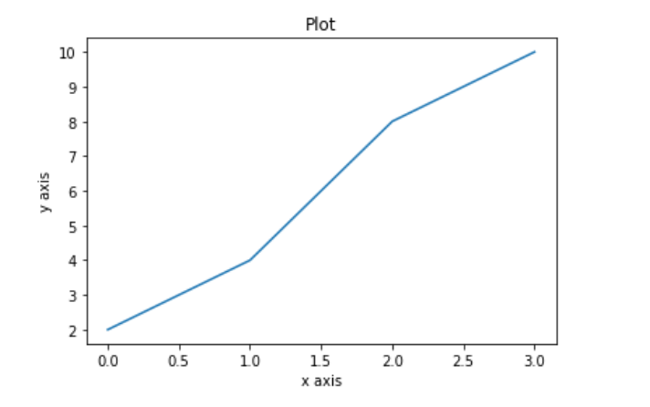
Basic Plot

plt.plot() and it drew a line chart automatically. The plt.plot accepts 3 basic arguments in the following order: (x, y, format). The creation of line chart was due it default behavior.

plt.xlabel() provides label to x-axis and plt.ylabel() provides label to the y-axis. plt.title() is used to define a title for the plot.

plt.plot([1,2,3,4,5], [2,2.5,3.5,6,8], 'o')
plt.show()

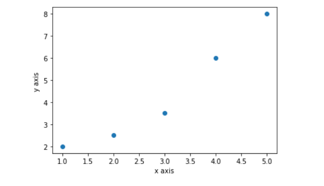
Basic scatterplot

The above code snippet shows the plotting of a scatter plot using format as 'o' which creates the dot on the provided axis points. The color blue is the default color.

fig, axes = plt.subplots(1,1, figsize=(10,6), sharex=True, sharey=True, dpi=120)

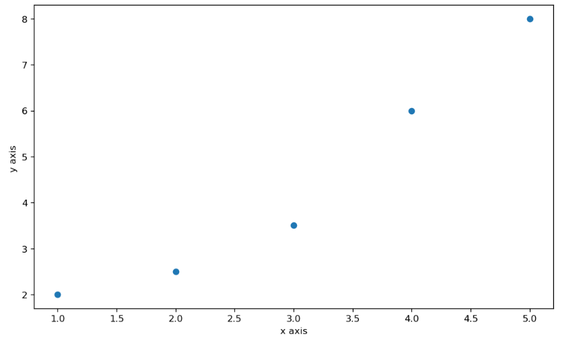
Figure size

fig, axes = plt.subplots(figsize()) changes the size of the plot

Matplotlib also comes with prebuilt colors and palettes. Type the following in your jupyter/python console to check out the available colors. However, these are base colors. Different colors can be used using different alphabets:

• r : represents red color
• k : represents black color
• g : represents green color
• c : represents cyan color
• b : represents blue color
• y : represents yellow color
• w : represents white color
• m : represents magenta color

plt.plot(1, 1, 'go') # green dots
plt.plot(2, 2, 'b*') # blue stars
plt.plot(2,6,'r*') #red asterisk
plt.plot(3,5, 'k^') #black upper triangle symbol
plt.plot(3,2,'cv') #cyan lower triangle symbol
plt.plot(2,4,'b+') #blue sum symbol
plt.plot(1,5,'m.') #magenta dot symbol
plt.show()

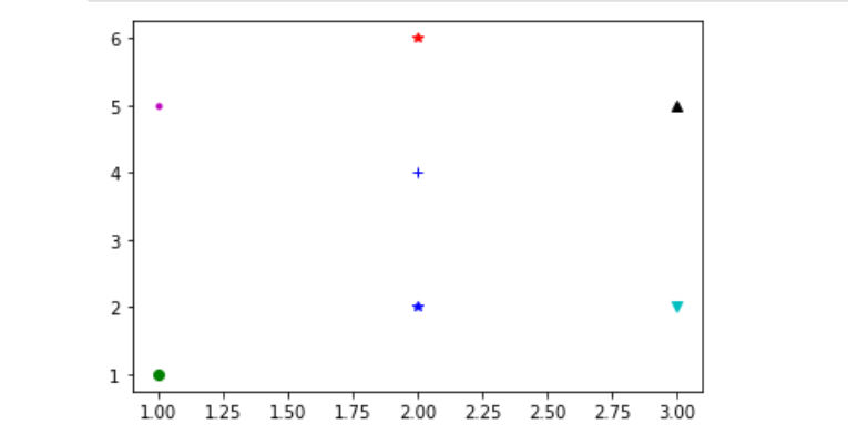
Plotting using markers

Basic Line Plot

a = range(100)
b = [value ** 4 for value in a]
plt.plot(a, b,'r')
plt.xlabel("x axis")
plt.ylabel("y axis")
plt.show()

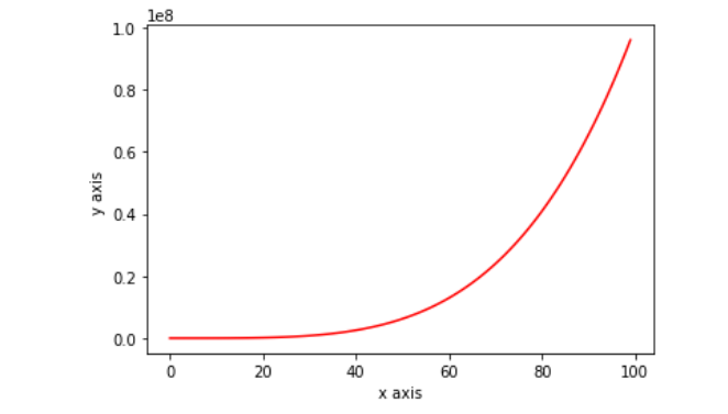
Line Plot

Plotting multiple curves

import numpy as np
X = np.linspace(0, 4 * np.pi, 100)
Ya = np.tan(X)
Yb = np.sin(X)
plt.plot(X, Ya)
plt.plot(X, Yb)
plt.show()

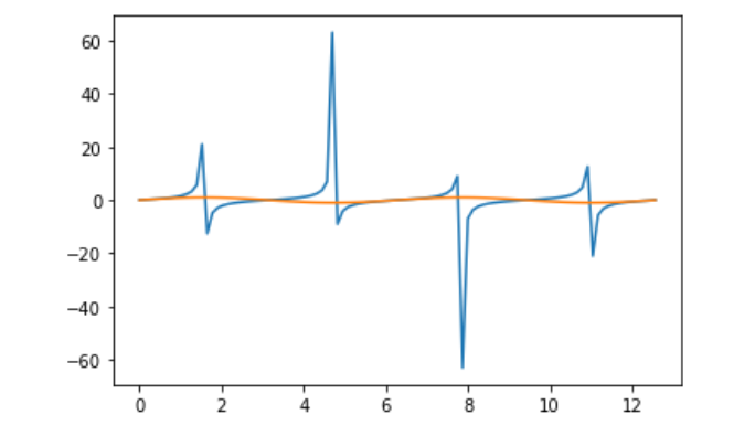
Multiple Curves

import numpy as np imports the Numpy Python library which is used for mathematical computations.

When displaying a curve, we implicitly assume that one point follows another, our data is the time series. Of course, this does not always have to be the case. One point of the data can be independent from the other. A simple way to represent such kind of data is to simply show the points without linking them.

Plotting points

df = np.random.rand(122, 4)
plt.scatter(df[:,0], df[:,1])
plt.show()

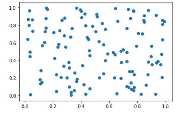
Plotting points

Bar Charts

Bar charts can be plotted by using pyplot.bar()  function.

df1 = [5, 12., 10., 8.]
plt.bar(range(len(df1)), df1)
plt.show()

For each value in the list data, one vertical bar is shown. The pyplot.bar()  function. receives two arguments—the x coordinate for each bar and the height of each bar. Here, we use the coordinates 0, 1, 2, and so on, for each bar, which is the purpose of range(len(data)) .

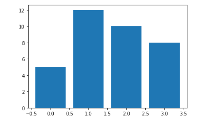
Bar Chart

Plotting multiple bar charts

When comparing several quantities and when changing one variable, we might want a bar chart where we have bars of one color for one quantity value.

data = np.arange(4)
plt.bar(df1 + 0.00, data[1], color = 'y', width=0.25)
plt.bar(df1 + 0.25, data[2], color = 'g', width=0.25)
plt.bar(df1 + 0.50, data[3], color = 'c', width=0.25)
plt.show()

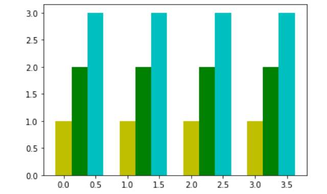
Multiple Bar Chart

Plotting stacked bar charts

Stacked bar charts are created by using a special parameter from pyplot.bar()  function of Matplotlib. The optional bottom parameter of the pyplot.bar()  function. allows you to specify a starting value for a bar. Instead of running from zero to a value, it will go from the bottom to value. The first call to pyplot.bar()  plots the cyan bars. The second call to pyplot.bar()  plots the magenta bars, with the bottom of the magenta bars being at the top of the cyan bars.

x = [2., 15., 25., 12.]
y = [3., 15., 30., 10.]
X = range(4)
plt.bar(X, x, color = 'c')
plt.bar(X, y, color = 'm', bottom = x)
plt.show()

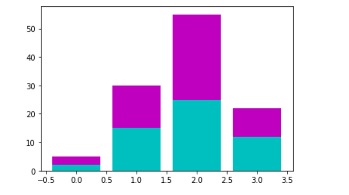
Stacked Bar Chart

Using custom colors for bar charts

Bar charts are used a lot in web pages and presentations where one often has to follow an established color scheme. Thus, a good control on their colors is a must.

boys = np.array([4., 3., 8., 12.,15.])
girls = np.array([1., 25., 7., 5.,6.])
Data = np.arange(5)
plt.barh(Data, boys , color ='0.55')
plt.barh(Data, -girls, color = '0.75')
plt.show()

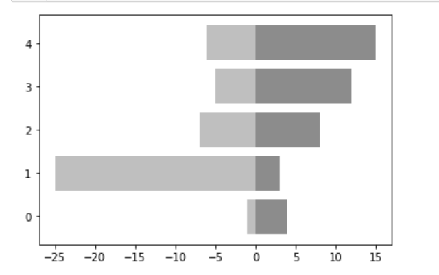
Customized Bar Chart

The pyplot.bar() and pyplot.barh()functions work strictly like pyplot.scatter() . We simply have to set the optional parameter color.

Boxplots

Boxplot allows you to compare distributions of values by conveniently showing the median, quartiles, maximum, and minimum of a set of values.

a = np.random.randn(50)
plt.boxplot(a)
plt.show()

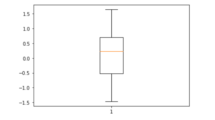
Box Plot

The data = [random.gauss(0., 1.) for i in range(50)] variable generates 50 values drawn from a normal distribution. For demonstration purposes, such values are typically read from a file or computed from other data.

The plot.boxplot() function takes a set of values and computes the mean, median, and other statistical quantities on its own. The following points describe the preceding boxplot:

. The red bar is the median of the distribution.

. The blue box includes 50 percent of the data from the lower quartile to the upper quartile. Thus, the box is centered on the median of the data

. The lower whisker extends to the lowest value within 1.5 IQR from the lower quartile.

. The upper whisker extends to the highest value within 1.5 IQR from the upper quartile.

. Values further from the whiskers are shown with a cross marker.

Pie Charts

Pie charts can be created by using the pie()  function.

import matplotlib.pyplot as plt
labels = 'Apples', 'Oranges', 'Bananas', 'Strawberries'
sizes = [35, 30, 25, 10]
fig, ax = plt.subplots()
ax.pie(sizes, explode=explode, labels=labels, autopct='%1.1f%%',shadow=True, startangle=90)
plt.show()

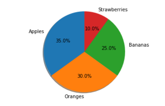
Pie Chart

Conclusion

Congratulations if you reached this far. Because we literally started from scratch and covered the essential topics to making matplotlib plots.

We covered the syntax and overall structure of creating matplotlib plots, saw how to modify various components of a plot, customized subplots layout, plots styling, colors, palettes, draw different plot types etc.